Creating complex balanced experimental designs need not be difficult. In this post I am introducing designr, an R package that has gradually developed over the past year. It simplifies creating complex factorial designs while making use of crossed/nested fixed/random factor specifications and generates complete experimental codes at the level of single observations by balancing conditions across experimental units (e.g., subjects and items) and vice versa.
Imagine you are about to plan a psychological study. Your theoretical framework and hypotheses will lead you to a number of conditions that you want to manipulate and present to subjects in order to analyze their responses later on. Many statistical tests will require that data are balanced, i.e. there should be an equal number of observations within each group. In many cases, this might be comparably easy but it can also become tricky with more factors and levels, some of which might be manipulated between/within subjects/items.
Is there an optimal way to ensure balancedness? Probably, no way is really perfect but some might be more practical than others. As part of my research projects over the past years I often needed to plan experiments in which not only the assignment of subjects to conditions is balanced but also that of items. Things can get tricky when some of the factors in the design are manipulated between subject but within item, the other way around or if all conditions are manipulated within subjects and within items but each pairing of subject and item is only to occur in one of several conditions and those assignments need to be balanced as well.
In an early version of what I am presenting here, I only had maybe ~150 lines of code. It was an R function that took (1) fixed factor names along with their levels, as well as lists of factor names that were (2) between subjects rather than within subjects and (3) between items rather than within items. However, the options were very limited and the handling was not very intuitive. To make it more flexible, I needed to add more and more arguments which made it even less straightforward. So I took some parts of the old code and write a couple hundred lines more. The idea was to tweak R’s internal syntax into something useful for creating experimental designs, so that the effort for the user is minimal, both for simple and complex designs.
Installing designr
The package is available on CRAN and can be installed just like most other packages:
install.packages("designr")
Once the package is installed, at the beginning of your code, you will need to load the package into your workspace by executing:
library(designr)
General handling: Factor plus factor equals design.
The main idea is this: What mainly distinguishes less complex from more complex designs is probably the number of factors in the design, i.e. the number of experimental manipulations, treatment levels, ect. In other words, you can always make a design more complex by adding another factor. The easiest design that is not just nothing has just one condition with one observation. Every factorial design can be derived from that by successively adding factor after factor. With designr, you can make use of that: To create a design from scratch, say design1, you can just add factors to each other with a plus sign:
design1 <- factor1 + factor2 + factor3 + ...
As usual for R, the expressions are parsed from left to right. So in the example above, first factor1 is evaluated, then factor2 is evaluated and added to factor1 to form a factorial design. When R encounters factor3, it is consequently added to the design. By loading the package, R learns what to do when it encounters factors and designs merged by the + operator.
With a design ready, you can also create a new one by just adding a factor like this:
design2 <- design1 + factor4
You will see later on what you can do with the resulting design objects (i.e., design1 or design2 in this example). But before you can handle the output, let’s have a closer look at the “input”: Fixed and random factors.
Factor definitions in designr
A factorial design consists of factors. Each factor can have different levels. Any factor whose levels are known beforehand (i.e., “fixed”), such as but not limited to (quasi-)experimental independent variables, is a fixed factor. This is the most common type of factor. You can easily define factors as follows and add them to each other to create a crossed design in which each level of the first factor can cooccur with each level of the other factor:
design <- fixed.factor("instruction", levels = c("A", "B")) + fixed.factor("difficulty", levels = c("low", "high"))
By adding the two factors instruction and difficulty, a design is created and stored in design. Every time a factor is added to a design, designr immediately updates the “codes”, a list of planned observations. You can either directly access it by design@design or by (what is recommended) using designr‘s output.design function, which comes with a variety of grouping/sorting options for the code matrix:
output.design(design)
The function prints a lot of useful information but the most important part is listed under $codes:
  instruction difficulty
1           A        low
2           B        low
3           A       high
4           B       high
As intended, we can see that the design requires 4 observations, one for each combination of instruction and difficulty. To explore what is possible in designr regarding the definition of factors, you can either check out the built-in manual/documentation pages or the Shiny app (click here) that lets you add different types of factors and shows you the R code you can just copy-and-paste and a preview of the design codes.
Nested and random factors
Some factors in your design might be nested within other factors. In that case, each level of the one factor cooccurs with only one level of the other factor. Or they can be crossed (which is the default), i.e. each level can cooccur with any level of the other factor. In psychology and other social sciences, nesting is often found with between-subject manipulations. If a manipulation is between subjects, i.e. each subject is assigned to only one level of the factor, subjects are nested within levels of the manipulation.
Subjects are a so-called random factor. That means, that the levels of the factor “subject” (i.e., the individual subjects) are not predefined by the design. In designr, you can add subjects as a random factor. Naturally, you don’t define the levels for the factor (designr will do that for you) but you just let designr know its name:
design <- fixed.factor("instruction", levels = c("A", "B")) + fixed.factor("difficulty", levels = c("low", "high")) + random.factor("Subject")
When you check the design output as before (using , you will see that there is an additional column Subject, which is 1 for all observations. That is because we haven’t told designr yet that the type of instruction is actually manipulated between subjects. We can do that by adding the groups argument:
design <- fixed.factor("instruction", levels = c("A", "B")) + fixed.factor("difficulty", levels = c("low", "high")) + random.factor("Subject", groups="instruction")
When you check the output, you will see that there are now 2 subjects and each one is assigned to only one of the instruction conditions but both difficulty conditions:
  instruction difficulty Subject
1           A        low       1
2           A       high       1
3           B        low       2
4           B       high       2
The package will determine a minimal number of levels for the random factor, i.e. a minimum number of subjects to be tested. The real number of subjects should be any multiple thereof if you want to keep the design complete. That number will mainly depend on the factors in which the random factor (the factor “subject”) is nested. The more between-subject manipulations you have, the more subjects you need in order to have a completely balanced experimental design.
Crossed random factors
Oftentimes, R packages that assist in designing experiments only consider at most one random factor (namely subjects, or none at all). In many cases, especially when you are not particularly interested in performing mixed model analyses, that approach might be sufficient. But if you are working with many different stimuli, for example, each of them could have a unique effect that is not captured (controlled for) in your fixed effects. Those cases are just one example for which it is useful to not only balance the assignment of subjects to conditions but also of items.
The designr package lets you define as many random factors as you like. You could also completely leave them out if they play no major role for your design. However, let’s consider that in the design outlined above, the difficulty in the experiment is mainly driven by two types of stimuli, so that difficulty remains a within-subject factor (i.e., we want each subject to see difficult and easy items) but at the same time it is a between-item factor (i.e., each item can only be difficult or easy). The type of instruction subjects receive remains a between-subject factor (because subjects only get one of the two instructions) but a within-item factor (because any item can appear under any instruction condition). The design can be created as follows:
design <- fixed.factor("instruction", levels = c("A", "B")) + fixed.factor("difficulty", levels = c("low", "high")) + random.factor("Subject", groups="instruction") + random.factor("Item", groups="difficulty")
By looking at the design output, we see that there are still two subjects but now to each difficulty condition (for both subjects, that is for both instruction conditions) one item is assigned:
output.design(design, order_by="Subject")$codes
  difficulty instruction Subject Item
1       high           A       1    1
2        low           A       1    2
3       high           B       2    1
4        low           B       2    2
Of course, this is a very sparse design so far. One way to increase the number of subjects and items would be to just “replicate” the random factors. For example, you could just change the definition of the Subject factor to random.factor("Subject", groups="instruction", replications=2) in order to double the number of subjects. Another way is to just add more fixed factors to the design, ideally those that play a role or are to be controlled for anyway.
Consider that in the experiment we are planning, no matter what instruction subjects are receiving, the task is always the same, namely to categorize the items. For each item, there is a correct response (X, Y, or Z). Oftentimes, you would like to have each of the three responses be correct exactly one third of the time to be able to distinguish a subject’s responses from chance. Our additional factor correct response is varied within subject but between item:
design <- fixed.factor("instruction", levels = c("A", "B")) + fixed.factor("difficulty", levels = c("low", "high")) + fixed.factor("correct_response", levels=c("X", "Y", "Z")) + random.factor("Subject", groups="instruction") + random.factor("Item", groups=c("difficulty", "correct_response"))
Looking at our design output output.design(design, order_by="Subject")$codes, we see that the design stay basically the same but we have 3-times as many items now and subjects are seeing exactly 3 difficult and 3 easy ones, as well as one for each condition of correct response within those difficulty levels:
   difficulty correct_response instruction Subject Item
1        high                X           A       1    1
2        high                Y           A       1    3
3        high                Z           A       1    5
4         low                X           A       1    2
5         low                Y           A       1    4
6         low                Z           A       1    6
7        high                X           B       2    1
8        high                Y           B       2    3
9        high                Z           B       2    5
10        low                X           B       2    2
11        low                Y           B       2    4
12        low                Z           B       2    6
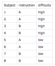
If we decided that subjects should also only see items from either difficulty instead of both, we could make difficulty a grouping (between-subject) factor for Subject and will see that we now need more subjects and every subject will only see the items from the difficulty group to which that subject was assigned:
design <- fixed.factor("instruction", levels = c("A", "B")) + fixed.factor("difficulty", levels = c("low", "high")) + fixed.factor("correct_response", levels=c("X", "Y", "Z")) + random.factor("Subject", groups="instruction") + random.factor("Item", groups=c("difficulty", "correct_response"))
   difficulty correct_response instruction Subject Item
1        high                X           A       1    1
2        high                Y           A       1    3
3        high                Z           A       1    5
4        high                X           B       2    1
5        high                Y           B       2    3
6        high                Z           B       2    5
7         low                X           A       3    2
8         low                Y           A       3    4
9         low                Z           A       3    6
10        low                X           B       4    2
11        low                Y           B       4    4
12        low                Z           B       4    6
The output.design function also provides you with information about the experimental units (levels of random factors) in the created design. You can access it through the $units entry of the list generated by output.design. In the current design, it contains the following:
$Subject
  Subject instruction difficulty
1       1           A       high
2       2           B       high
3       3           A        low
4       4           B        low

$Item
  Item difficulty correct_response
1    1       high                X
2    2        low                X
3    3       high                Y
4    4        low                Y
5    5       high                Z
6    6        low                Z
As you can see, for each random factor (Subject and Item), there is a data frame with the factor level and the groups to which that Subject or Item is assigned. Once the design is created, this can serve as a helpful reference to assign real subjects to sessions/versions or to generate a stimulus set.
Constraining random factor interactions
Consider an experiment like the one we have used as an example so far but every subject sees every item in a condition that is designed to occur for every subject (i.e., a within-subject factor) and for every item (i.e., a within-item factor). For example, for 50% of the trials, we want the prompt appearing on the screen to be phrased differently. Theoretically, you would just add that fixed factor to the design like this:
design <- fixed.factor("instruction", levels = c("A", "B")) + fixed.factor("difficulty", levels = c("low", "high")) + fixed.factor("correct_response", levels = c("X", "Y", "Z")) + random.factor("Subject", groups = "instruction") + random.factor("Item", groups = c("difficulty", "correct_response")) + fixed.factor("phrasing", levels = c("positive", "negative"))
This is, of course, not an issue for designr. However, when you look at the first lines of design codes, you will notice that the items for subject 1 appear twice: once in the positive and once in the negative phrasing condition:
   difficulty correct_response instruction Subject Item phrasing
1        high                X           A       1    1 positive
2        high                Y           A       1    3 positive
3        high                Z           A       1    5 positive
4         low                X           A       1    2 positive
5         low                Y           A       1    4 positive
6         low                Z           A       1    6 positive
7        high                X           A       1    1 negative
8        high                Y           A       1    3 negative
9        high                Z           A       1    5 negative
10        low                X           A       1    2 negative
11        low                Y           A       1    4 negative
12        low                Z           A       1    6 negative
13       high                X           B       2    1 positive
...
There are possible scenarios in which this could be very useful, of course. However, what if you want each item-subject pairing to appear only once? In other words, how do you ensure that the items that are assigned to a subject are only assigned once and only under either phrasing condition?
design <- fixed.factor("instruction", levels = c("A", "B")) + fixed.factor("difficulty", levels = c("low", "high")) + fixed.factor("correct_response", levels = c("X", "Y", "Z")) + random.factor("Subject", groups = c("instruction", "difficulty")) + random.factor("Item", groups = c("difficulty", "correct_response")) + fixed.factor("phrasing", levels = c("positive", "negative")) + random.factor(c("Subject","Item"), groups = "phrasing")
In designr, you can do so by nesting the interaction of the random factors Subject and Item within the fixed factor phrasing. Depending on the rotation mechanism used (Latin square by default), this will also increase the number of subjects and items and ensure that not only the balancedness so far remains intact but also that all item and subject groups appear equally often with both phrasing conditions, and vice versa. And most importantly, it also ensures that each individual subject and each individual item, across the entire set of design codes/planned observations, appear equally often in all conditions, including the new phrasing condition.
Using the designr factor syntax
You can use designr mainly in two different ways: You can either create factors using the functions fixed.factor or random.factor and add them to create a design object, or you pass a factor formula to factor.design. Even though this is fully optional and therefore unnecessary to look into, it can save you a couple of keystrokes and maybe even simplify things.
Looking at the design specification from above:
# Note: line breaks are not necessary
design <- fixed.factor("instruction", levels = c("A", "B")) +
          fixed.factor("difficulty", levels = c("low", "high")) +
          fixed.factor("correct_response", levels = c("X", "Y", "Z")) +
          random.factor("Subject", groups = c("instruction", "difficulty")) +
          random.factor("Item", groups = c("difficulty", "correct_response")) +
          fixed.factor("phrasing", levels = c("positive", "negative")) +
          random.factor(c("Subject","Item"), groups = "phrasing")
… you can write the same design a little bit shorter as follows:
# Note: line breaks are not necessary
design <- factor.design( ~
    instruction(A,B) +
    difficulty(low,high) +
    correct_response(X,Y,Z) +
    Subject[instruction, difficulty] +
    Item[difficulty, correct_response] +
    phrasing(positive,negative) +
    Subject:Item[phrasing]
)
In R, anything with the tilde operator ~ is interpreted as a “formula”. You may have seen that with analysis functions such as lm or lmer. In designr, I am using that feature for interpreting experimental designs. All this is doing is translating that “factor syntax” to the fixed.factor and random.factor function calls above but some users might find this easier to look at.
A factor definition always starts with the name. If parentheses ((...)) follow, it is interpreted as a fixed factor with the levels specified inside the parentheses. This can also be a numeric range such as 3:5 (which expands to 3, 4, and 5 in R). If no parentheses follow the factor name, it is interpreted as a random factor (as random factors do not have predefined levels). To nest the fixed or random factor within previously defined factors, you can list the factor names that define the groups in brackets ([...]) .
Hands-on exploration of designr with Shiny
If you are not yet convinced or would like a more hands-on introduction, I have prepared a Shiny app. There is no need to install anything (not even R) to test this, so there is no harm in looking here. You can select “designr blog example” from the example list to populate inputs with values that let you replicate the example in this blog post. Or you can just start from scratch with your own design. The app does not only show you the design code matrix but also produces the R code you can copy-and-paste into your own R session to replicate the same design on your own computer.
More output and saving options
As mentioned above, every time you add a factor, the design is extended by the levels of that factor, respecting the specified constraints, if applicable. Once your design is complete, or at any time in between, you can let designr create a copied output version of your design to look at in R, use in any way you like or even write to a set of output files to use directly in your experimental software.
The function output.design lets you specify the arguments group_by, order_by, and randomize. You can look up the manual page for more details but an example call to create useful output in which the codes are grouped by subjects and randomly shuffled within each subject would be:
output.design(design, group_by="Subject", randomize=T)
You can also group by multiple columns and sort the output within each group by any other columns in your design matrix. The random shuffling (if set to TRUE) takes place within each group and before sorting.
Additionally, you can directly write your design into files. You can also use grouping, sorting and randomizing. By default, for each output group, one “run” file is created, in which the experimental codes for that output group (subject in our case) are written out. Additionally, codes and condition assignments for each random factor are written out as well. That way, you can easily output your design for use in other software.
There is a general write.design function which requires you to specify an output handler (such as write.csv). Said output handler should be a function that accepts a data frame as a first argument and a file name as a second argument. All arguments passed to write.design that are not interpreted by write.design directly, are passed on as additional arguments to the output handler. Alternatively, you can also use the built-in default functions write.design.csv or write.design.json, which are wrapper functions for write.design but by default use utils::write.csv and jsonlite::write_json as output handlers.
For example, the command write.design.csv(design, group_by="Subject", randomize=T) creates 8 run files (run*.csv) and 3 random factor assignment files (codes*.csv):

Each run*.csv file contains a randomly shuffled sequence of trials with a header line and 6 planned observations (one in each phrasing × correct_response condition but all in the same difficulty × instruction condition because those are constant for each subject:

In codes_Subject.csv, for example, we find a list of all planned subjects. And of course, for subject 5, we see the assignment to instruction A and low difficulty, as we can also see in run_Subject-5.csv above.
You could also consider grouping along more columns than Subject. In that case, more run*.csv files are generated. If no grouping at all is used, only one single run.csv is created.